Sequential Monte Carlo

Sequential Monte Carlo (SMC) is a general extension of particle filtering, which provides a flexible sampling framework for computing the posterior distribution of nonlinear state-space models.

Nonlinear state space model

Suppose we have a nonlinear state space model

where $\mathrm{\theta}$ denotes the hyperparameter of the dynamics. We are interested in the inference of the model to understand the dynamics. To that end, we compute the marginal likelihood of the model

where each sub-component of the marginal likelihood follows that

where \(\mathrm{\mathbf{x}^{(i)}_{t}\sim p(\mathbf{x}_{t} \\| \mathbf{y}_{1:t-1},\theta)}\). To simulate the desired set of particles \(\{\mathrm{\mathbf{x}_{t}^{(i)}}\}_{i=1}^N\), we observe that

Suppose a set of particles \(\{\mathrm{\mathbf{x}_{t-1}^{(i)}}\}_{i=1}^N\), where \(\mathrm{\mathbf{x}^{(i)}_{t-1}\sim p(\mathbf{x}_{t-1} \\| \mathbf{y}_{1:t-2},\theta)}\), is available. The above relation inspires to us to design an algorithm as follows

Algorithm

Sample weights

Given the particles \(\{\mathrm{\mathbf{x}_{t-1}^{(i)}}\}_{i=1}^N\), compute the sample weight for resampling and likelihood estimation

Likelihood estimation

Approximate the likelihood at time $t-1$ following \eqref{marginal_approximation}, where a more refined version regarding the log likelihood is presented in (Andrieu et al., 2004)

Resampling

Normalize $\mathrm{w_{t-1}^{(i)}}$ into \(\mathrm{\overline w_{t-1}^{(i)}}\propto \mathrm{w_{t-1}^{(i)}} \propto \mathrm{p(\mathbf{y}_{t-1} \\| \mathbf{x}^{(i)}_{t-1},\theta)}\), s.t. $\mathrm{\sum_{i=1}^N\overline w_{t-1}^{(i)}=1}$.

Resample the particles \(\{\mathrm{\mathbf{x}_{t-1}^{(i)}}\}_{i=1}^N\) according to the probability $\mathrm{\overline w_{t-1}^{(i)}}$.

Propagation

Draw a set of new particles following the dynamics

The algorithm described above is the bootstrap particle filter, which employs a proposal distribution identical to the propagation step and performs resampling at every step. To simulate the desired particles following Eq. \eqref{latent_simulate}, we adopt a slightly different ordering:

\(\begin{align} \cdots \rightarrow \underbrace{\text{sample weight}\rightarrow \text{resampling}}_{\mathrm{p(\mathbf{y}_{t-1} \\| \mathbf{x}^{(i)}_{t-1},\theta)}}\rightarrow \underbrace{\text{propagation}}_{\mathrm{p(\mathbf{x}^{(i)}_t|\mathbf{x}^{(i)}_{t-1}, \theta) }} \rightarrow \cdots \end{align}\) This ordering can be naturally adjusted to standard formulations, as studied in Section 16.3.5 (Särkkä, 2023) and (Alenlöv, 2019-08-26). Additionally, for simplicity, we do not explicitly introduce the concept of (sequential) importance sampling in this presentation. We will introduce proposal-optimized variates of SMC for future blogs.

Combining Eq.\eqref{marginal_pdf} and \eqref{unbiased_conditional_Z}, we observe the marginal likelihood can be estimated as follows

where the unbiased property of \(\mathrm{\widetilde Z}\) has been studied in (Andrieu et al., 2010).

Stochastic volatility models in finance

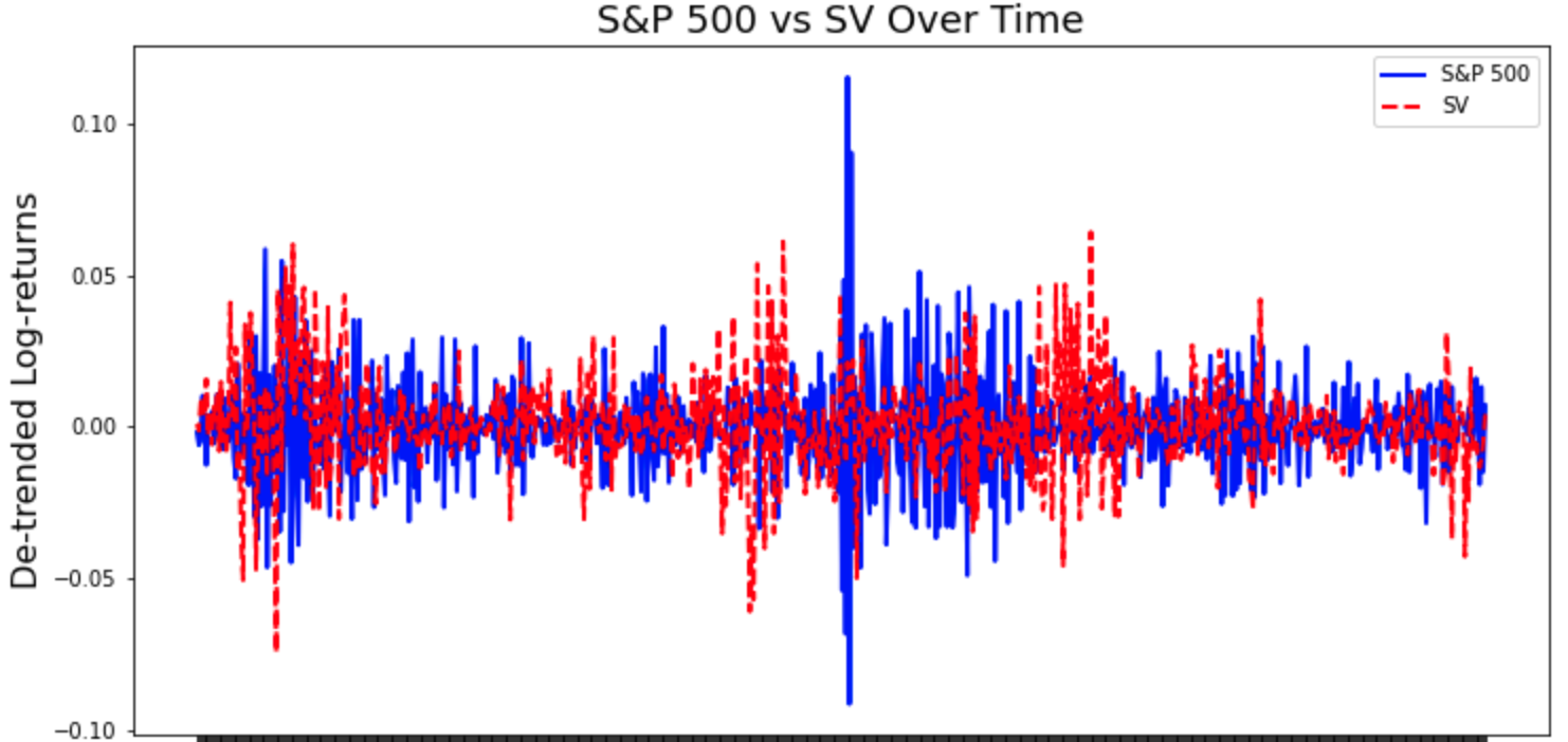
Stochastic volatility (SV) models are popular in finance to model the dynamics of heteroskedastic financial assets to hedge risks (Creal, 2012). Consider a SV model (Doucet & Johansen, 2011)

where $\mathrm{y_t}$ denotes the S&P 500 log-return data.

The following code snippet is an example on the SV model from (Kviman et al., 2024)

class SV:
    def __init__(self, sigma=1., beta=.1, phi=0.99):
        self.sigma = sigma
        self.beta = beta
        self.phi = phi

    def particle_0(self, N):
        return np.random.normal(0, self.sigma / np.sqrt(1 - self.phi ** 2), size=(N, 1))

    def propagate(self, x):
        x_next = self.phi * x.squeeze() + self.sigma * npr.normal(size=x.size)
        return x_next.reshape((-1, 1))

    def log_g(self, x, y):
        return stats.norm.logpdf(y, loc=0, scale=np.sqrt(self.beta**2 * np.exp(x))).squeeze()

The resampling schemes (Naesseth et al., 2019) include the standard multinomial resampling and stratified (or systematic) resampling for variance reduction.

def multinomial_resampling(ws, size=0):
    u = np.random.rand(*ws.shape)
    bins = np.cumsum(ws)
    return np.digitize(u, bins)


def stratified_resampling(ws, size=0):
    N = len(ws)
    u = (np.arange(N) + np.random.rand(N)) / N
    bins = np.cumsum(ws)
    return np.digitize(u, bins)

The marginal log likelihood estimation can be conducted as follows

def bootstrap_filter(model, y, N, T, d, resampling, update_weights):
    # Initialize storage arrays
    particles = np.zeros((N, d, T))
    normalized_weights = np.zeros((N, T))
    log_weights = np.zeros((N, T))
    
    # Initialize marginal log-likelihood
    marg_log_likelihood = 0.0

    # Initial particles and weights
    particles[..., 0] = model.particle_0(N)
    log_g_t = model.log_g(x=particles[:, :d_y, 0], y=y[0])
    normalized_weights[:, 0], log_weights[:, 0] = update_weights(log_weights[:, 0], log_g_t)
    
    marg_log_likelihood += logsumexp(log_weights[:, 0]) - np.log(N)

    for t in range(1, T):
        # Resampling at every step
        new_ancestors = resampling(normalized_weights[:, t - 1]).astype(int)
        normalized_weights[:, t - 1] = 1 / N  # Reset weights after resampling
        log_weights[:, t - 1] = 0

        # Propagate particles
        particles[:, :, t] = model.propagate(particles[new_ancestors, :, t - 1])

        # Compute weights
        log_g_t = model.log_g(particles[:, :d_y, t], y[t])
        normalized_weights[:, t], log_weights[:, t] = update_weights(log_weights[:, t - 1], log_g_t)

        # Update marginal log-likelihood
        marg_log_likelihood += logsumexp(log_weights[:, t]) - np.log(N)

    return particles, normalized_weights, log_weights, marg_log_likelihood

def update_weights(log_weights, log_g_t):
    log_weights += log_g_t
    log_w_tilde = log_weights - logsumexp(log_weights)
    normalized_weights = np.exp(log_w_tilde)
    return normalized_weights, log_weights

The simulations below effectively capture the clustering effect of volatility for the daily log-returns of S&P 500. We acknowledge that there are still limitations in this model, such as the inefficacy to tackle the long-term dependencies, heavy tails, or high dimensional problems, but this is a good start to understand nonlinear state space models.