A coupling of two random variables/ vectors represents a joint distribution, where the marginal distributions are denoted by $p$ and $q$, respectively. Any joint distributions of $p$ and $q$ define a valid coupling. Although there are infinitely many of them, some of them are quite special and may facilitate our analysis.

Maximal Coupling

Total variation distance is defined as follows

$$\mathrm{\forall }\mathrm{A}\in \mathrm{X},|\mathrm{p}-\mathrm{q}{|}_{\text{TV}}=\underset{\mathrm{X}\in \mathrm{A}}{sup}\mathbb{P}(\mathrm{X}\in \mathrm{A})-\mathbb{P}(\mathrm{Y}\in \mathrm{A}),$$ where $\mathrm{X}$ and $\mathrm{Y}$ are random variables defined on the state space $\mathbb{X}$ with measurable set $X$. Note that for any measurable set $\mathrm{A}\in \mathrm{X}$, the follow inequality always holds

$\mathbb{P}(\mathrm{X}\in \mathrm{A})-\mathbb{P}(\mathrm{Y}\in \mathrm{A})=\mathbb{P}(\mathrm{X}\in \mathrm{A}\cap \mathrm{X}\ne \mathrm{Y})-\mathbb{P}(\mathrm{Y}\in \mathrm{A}\cap \mathrm{X}\ne \mathrm{Y})\le \mathbb{P}(\mathrm{X}\ne \mathrm{Y})$.

There exists one pair of $(\mathrm{X},\mathrm{Y})$ such that the above inequality holds. Any coupling that satisfies this property is known as maximal coupling.

Denoting by $\nu =\mathrm{p}-\mathrm{q}$ the zero-mass measure, there is a set $D$ according to the Hahn-Jordan decomposition such that ${\nu }^{+}=(\mathrm{p}-\mathrm{q})(\cdot \cap \mathrm{D})$ and ${\nu }^{-}=(\mathrm{q}-\mathrm{p})(\cdot \cap {\mathrm{D}}^{\mathrm{c}})$ are both positive measures and $\nu ={\nu }^{+}-{\nu }^{-}$.

Notably, it is clear that $\mathrm{D}=\{\mathrm{x}:\mathrm{p}(\mathrm{x})\ge \mathrm{q}(\mathrm{x})\}$. It follows that $\underset{\mathrm{A}\in \mathrm{X}}{sup}\mathbb{P}(\mathrm{X}\in \mathrm{A})-\mathbb{P}(\mathrm{Y}\in \mathrm{A})=\underset{\mathrm{A}\in \mathrm{X}}{sup}\nu (\mathrm{A})=\nu (\mathrm{D})=\mathbb{P}(\mathrm{X}\in \mathrm{D})-\mathbb{P}(\mathrm{Y}\in \mathrm{D})$. We have

$$\begin{array}{rl}\mathbb{P}(\mathrm{X}\in \mathrm{D})-\mathbb{P}(\mathrm{Y}\in \mathrm{D})& ={\int }_{\{\mathrm{x}:\mathrm{p}(\mathrm{x})\ge \mathrm{q}(\mathrm{x})\}}\mathrm{p}(\mathrm{x})\mathrm{d}\mathrm{x}-{\int }_{\{\mathrm{x}:\mathrm{p}(\mathrm{x})\ge \mathrm{q}(\mathrm{x})\}}\mathrm{q}(\mathrm{x})\mathrm{d}\mathrm{x}\\ & ={\int }_{\{\mathrm{x}:\mathrm{p}(\mathrm{x})<\mathrm{q}(\mathrm{x})\}}\mathrm{q}(\mathrm{x})\mathrm{d}\mathrm{x}-{\int }_{\{\mathrm{x}:\mathrm{p}(\mathrm{x})<\mathrm{q}(\mathrm{x})\}}\mathrm{p}(\mathrm{x})\mathrm{d}\mathrm{x}.\end{array}$$

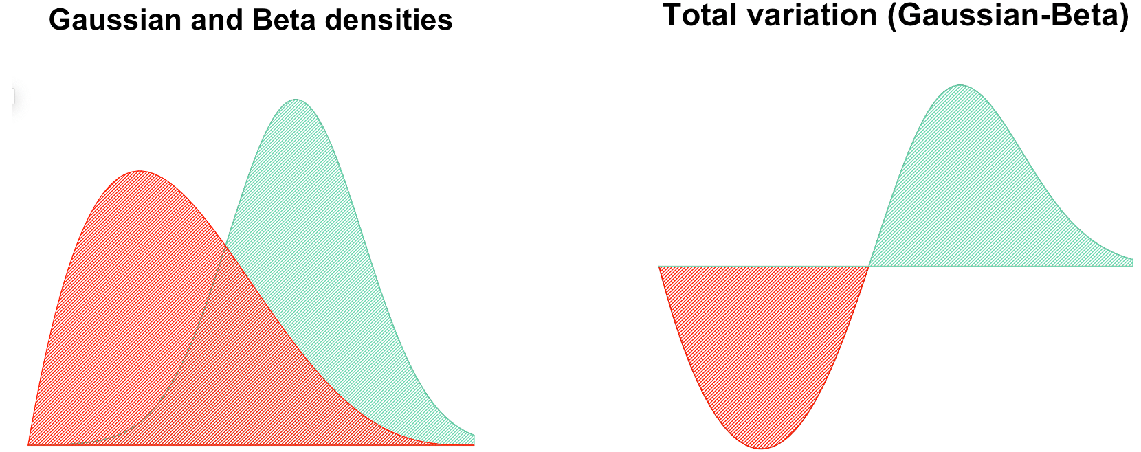
Summing up the above equations and combining $|a-b|=a+b-2a\wedge b$, we can obtain the area between the two pdf curves (Jacob, 2021)

$$|\mathrm{p}-\mathrm{q}{|}_{\text{TV}}=\frac{1}{2}\int |\mathrm{p}(\mathrm{x})-\mathrm{q}(\mathrm{x})|\mathrm{d}\mathrm{x}=1-\int min\{\mathrm{p}(\mathrm{x}),\mathrm{q}(\mathrm{x})\}\mathrm{dx}.$$

In the end, we can summarize the different formulations of total variation

$$\begin{array}{rl}\Vert \mathrm{p}-\mathrm{q}{\Vert }_{\text{TV}}& =sup\mathbb{P}(\mathrm{X}\in \mathrm{A})-\mathbb{P}(\mathrm{Y}\in \mathrm{A})\\ & =\frac{1}{2}\int |\mathrm{p}(\mathrm{x})-\mathrm{q}(\mathrm{x})|\mathrm{d}\mathrm{x}\\ & =1-\int min\{\mathrm{p}(\mathrm{x}),\mathrm{q}(\mathrm{x})\}\mathrm{d}\mathrm{x}\\ & =\underset{(\mathrm{X},\mathrm{Y})\in \text{coupling}(\mathrm{p},\mathrm{q})}{inf}\mathbb{P}(\mathrm{X}\ne \mathrm{Y}).\end{array}$$

Applications

Suppose $({\mathrm{X}}_{\mathrm{i}})$ follow an (independent) binomial distribution $\mathrm{Binomial}(\lambda ,\mathrm{N})$ and $({\mathrm{Y}}_{\mathrm{i}})$ follow an (independent) Poisson distribution $\mathrm{Poisson}(\lambda )$. Next, we couple ${\mathrm{X}}_{\mathrm{i}}$ and ${\mathrm{Y}}_{\mathrm{i}}$ maximally. The overlap mass is equal to $(1-\lambda )\wedge {\mathrm{e}}^{-\lambda }+\lambda \wedge \lambda {\mathrm{e}}^{-\lambda }=1-\lambda +\lambda {\mathrm{e}}^{-\lambda }$. That means $\mathbb{P}({\mathrm{X}}_{\mathrm{i}}\ne {\mathrm{Y}}_{\mathrm{i}})=\lambda (1-{\mathrm{e}}^{-\lambda })\le {\lambda }^2$.

Replace $\lambda$ with $\lambda /N$, we have $$\mathbb{P}\left(\frac{\sum _{\mathrm{i}=1}^{\mathrm{N}}{\mathrm{X}}_{\mathrm{i}}-\sum _{\mathrm{i}=1}^{\mathrm{N}}{\mathrm{Y}}_{\mathrm{i}}}{\mathrm{N}}\right)\le \frac{{\lambda }^2}{\mathrm{N}},$$ where implies that given a large N and a fixed $\lambda$, Poisson distribution approximates the binomial distribution.

Convergence rates

By assuming $({\mathrm{Y}}_{\mathrm{t}})$ is simulated from the stationary distribution in the beginning, we can introduce a coupling inequality such that

$$\mathrm{L}({\mathrm{X}}_{\mathrm{t}})-\mathrm{L}({\mathrm{Y}}_{\mathrm{t}})|\le \mathbb{P}(\tau >\mathrm{t}),$$ where $\tau$ is a random variable that enables ${\mathrm{X}}_{\mathrm{t}}={\mathrm{Y}}_{\mathrm{t}}$ and is also known as ‘‘meeting time’’. The equality can be achieved given the maximal coupling but the contruction may differ in different problems. In addition, meeting exactly sometimes is quite restricted; it is enough to consider close enough chains.

Synchronous Coupling

Synchronous coupling models the contraction of a pair of trajectories and can be used to prove the convergence of stochastic gradient Langevin dynamics for strongly log-concave distributions.

Let ${\theta }_{\mathrm{k}}\in {\mathbb{R}}^{\mathrm{d}}$ be the $k$-th iterate of the following stochastic gradient Langevin algorithm. $$\begin{array}{r}{\theta }_{\mathrm{k}+1}={\theta }_{\mathrm{k}}-\eta \mathrm{\nabla }\tilde{\mathrm{f}}({\theta }_{\mathrm{k}})+\sqrt{2\tau \eta }{\xi }_{\mathrm{k}},\end{array}$$ where $\eta$ is the learning rate, $\tau$ is the temperature, ${\xi }_{\mathrm{k}}$ is a standard $d$-dimensional Gaussian vector, and $\mathrm{\nabla }\tilde{\mathrm{f}}(\theta )$ is an unbiased estimate of the exact gradient $\mathrm{\nabla }\mathrm{f}(\theta )$.

Assumptions

Smoothness We say $\mathrm{f}$ is $\mathrm{L}$-smooth if for some $\mathrm{L}>0$ $$\begin{array}{}\text{(1)}& \mathrm{f}(\mathrm{y})\le \mathrm{f}(\mathrm{x})+⟨\mathrm{\nabla }\mathrm{f}(\mathrm{x}),\mathrm{y}-\mathrm{x}⟩+\frac{\mathrm{L}}{2}\Vert \mathrm{y}-\mathrm{x}{\Vert }_2^2\mathrm{\forall }\mathrm{x},\mathrm{y}\in {\mathbb{R}}^{\mathrm{d}}.\end{array}$$

Strong convexity We say $\mathrm{f}$ is $\mathrm{m}$-strongly convex if for some $\mathrm{m}>0$ $$\begin{array}{}\text{(2)}& \mathrm{f}(\mathrm{x})\ge \mathrm{f}(\mathrm{y})+⟨\mathrm{\nabla }\mathrm{f}(\mathrm{y}),\mathrm{x}-\mathrm{y}⟩+\frac{\mathrm{m}}{2}\Vert \mathrm{y}-\mathrm{x}{\Vert }_2^2\mathrm{\forall }\mathrm{x},\mathrm{y}\in {\mathbb{R}}^{\mathrm{d}}.\end{array}$$

Bounded variance The variance of stochastic gradient $\mathrm{\nabla }\tilde{\mathrm{f}}(\mathrm{x})$ is upper bounded such that $$\begin{array}{}\text{(3)}& \mathbb{E}[\Vert \mathrm{\nabla }\tilde{\mathrm{f}}(\mathrm{x})-\mathrm{\nabla }\mathrm{f}(\mathrm{x}){\Vert }^2]\le {\sigma }^2\mathrm{d},\mathrm{\forall }\mathrm{x}\in {\mathbb{R}}^{\mathrm{d}}.\end{array}$$

A Crude Estimate

Assume assumptions $\text{1}$, $\text{2}$, and $\text{3}$ hold. For any learning rate $\eta \in (0,1\wedge \mathrm{m}/{\mathrm{L}}^2)$ and $||{\theta }_0-{\theta }_{\ast }||\le \sqrt{\mathrm{d}}\mathrm{D}$, where ${\theta }_{\ast }$ is a stationary point. Then

$$\begin{array}{r}{\mathrm{W}}_2({\mu }_{\mathrm{k}},\pi )\le {\mathrm{e}}^{-\mathrm{mk}\eta /2}\cdot 2(\sqrt{\mathrm{d}}\mathrm{D}+\sqrt{\mathrm{d}/\mathrm{m}})+\sqrt{2\mathrm{d}({\sigma }^2+{\mathrm{L}}^2\mathrm{G}\eta )/{\mathrm{m}}^2},\end{array}$$

where ${\mu }_{\mathrm{k}}$ denotes the probability measure of ${\theta }_{\mathrm{k}}$ and $\mathrm{G}:=25(\tau +\mathrm{m}{\mathrm{D}}^2+{\sigma }^2)$.

Proof

Denote ${\theta }_{\mathrm{t}}$ as the continuous-time interpolation of the stochastic gradient Langevin dynamics as follows

$$\begin{array}{r}\mathrm{d}{\theta }_{\mathrm{t}}=-\mathrm{\nabla }\tilde{\mathrm{f}}({\theta }_{\eta \lfloor \frac{\mathrm{t}}{\eta }\rfloor })\mathrm{d}\mathrm{t}+\sqrt{2\tau }\mathrm{d}{\tilde{\mathrm{W}}}_{\mathrm{t}},\end{array}$$

where ${\theta }_0={\theta }_0$. For any $\mathrm{k}\in {\mathbb{N}}^{+}$ and a time $\mathrm{t}$ that satisfies $\mathrm{t}=\mathrm{k}\eta$, it is apparent that ${\hat{\mu }}_{\mathrm{t}}=\mathrm{L}({\theta }_{\mathrm{t}})$ is the same as ${\mu }_{\mathrm{k}}=\mathrm{L}({\theta }_{\mathrm{k}})$, where $\mathrm{L}(\cdot )$ denotes a distribution of a random variable. In addition, we define an auxiliary process $({\beta }_{\mathrm{t}})$ that starts from the stationary distribution $\pi$

$$\begin{array}{r}\mathrm{d}{\beta }_{\mathrm{t}}=-\mathrm{\nabla }\mathrm{f}({\beta }_{\mathrm{t}})\mathrm{d}\mathrm{t}+\sqrt{2\tau }\mathrm{d}{\mathrm{W}}_{\mathrm{t}}.\end{array}$$

Consider Itô’s formula for the sequence of $\frac{1}{2}\Vert {\theta }_{\mathrm{t}}-{\beta }_{\mathrm{t}}{\Vert }^2$

$$\begin{array}{rl}& \frac{1}{2}\mathrm{d}\Vert {\theta }_{\mathrm{t}}-{\beta }_{\mathrm{t}}{\Vert }^2\\ & =⟨{\theta }_{\mathrm{t}}-{\beta }_{\mathrm{t}},\mathrm{d}{\theta }_{\mathrm{t}}-\mathrm{d}{\beta }_{\mathrm{t}}⟩+\mathrm{Tr}[{\mathrm{d}}^2{\theta }_{\mathrm{t}}-{\mathrm{d}}^2{\beta }_{\mathrm{t}}]\\ & =⟨{\theta }_{\mathrm{t}}-{\beta }_{\mathrm{t}},(\mathrm{\nabla }\mathrm{f}({\beta }_{\mathrm{t}})-\mathrm{\nabla }\tilde{\mathrm{f}}({\theta }_{\eta \lfloor \frac{\mathrm{t}}{\eta }\rfloor }))\mathrm{d}\mathrm{t}+\sqrt{2\tau }(\mathrm{d}{\tilde{\mathrm{W}}}_{\mathrm{t}}-\mathrm{d}{\mathrm{W}}_{\mathrm{t}})⟩+2\tau \mathrm{Tr}[{\mathrm{d}}^2{\tilde{\mathrm{W}}}_{\mathrm{t}}-{\mathrm{d}}^2{\mathrm{W}}_{\mathrm{t}}].\end{array}$$

Taking ${\tilde{\mathrm{W}}}_{\mathrm{t}}={\mathrm{W}}_{\mathrm{t}}$ defines a synchronous coupling. Arrange the terms

$$\begin{array}{rl}& \frac{1}{2}\mathrm{d}\Vert {\theta }_{\mathrm{t}}-{\beta }_{\mathrm{t}}{\Vert }^2\\ & =⟨{\theta }_{\mathrm{t}}-{\beta }_{\mathrm{t}},\mathrm{\nabla }\mathrm{f}({\beta }_{\mathrm{t}})-\mathrm{\nabla }\mathrm{f}({\theta }_{\mathrm{t}})⟩\mathrm{d}\mathrm{t}+⟨{\theta }_{\mathrm{t}}-{\beta }_{\mathrm{t}},\mathrm{\nabla }\mathrm{f}({\theta }_{\mathrm{t}})-\mathrm{\nabla }\mathrm{f}({\theta }_{\eta \lfloor \frac{\mathrm{t}}{\eta }\rfloor })⟩\mathrm{d}\mathrm{t}\\ & +⟨{\theta }_{\mathrm{t}}-{\beta }_{\mathrm{t}},\mathrm{\nabla }\mathrm{f}({\theta }_{\eta \lfloor \frac{\mathrm{t}}{\eta }\rfloor })-\mathrm{\nabla }\tilde{\mathrm{f}}({\hat{\theta }}_{\eta \lfloor \frac{\mathrm{t}}{\eta }\rfloor })⟩\mathrm{d}\mathrm{t}\\ & \le -\mathrm{m}\Vert {\theta }_{\mathrm{t}}-{\beta }_{\mathrm{t}}{\Vert }^2\mathrm{d}\mathrm{t}+\frac{\mathrm{m}}{4}\Vert {\theta }_{\mathrm{t}}-{\beta }_{\mathrm{t}}{\Vert }^2\mathrm{d}\mathrm{t}+\frac{1}{\mathrm{m}}\Vert \mathrm{\nabla }\mathrm{f}({\theta }_{\mathrm{t}})-\mathrm{\nabla }\mathrm{f}({\theta }_{\eta \lfloor \frac{\mathrm{t}}{\eta }\rfloor }){\Vert }^2\mathrm{d}\mathrm{t}\\ & +\frac{\mathrm{m}}{4}\Vert {\theta }_{\mathrm{t}}-{\beta }_{\mathrm{t}}\Vert {\Vert }^2\mathrm{d}\mathrm{t}+\frac{1}{\mathrm{m}}\Vert \mathrm{\nabla }\mathrm{f}({\theta }_{\eta \lfloor \frac{\mathrm{t}}{\eta }\rfloor })-\mathrm{\nabla }\tilde{\mathrm{f}}({\hat{\theta }}_{\eta \lfloor \frac{\mathrm{t}}{\eta }\rfloor }){\Vert }^2\mathrm{d}\mathrm{t}\\ & \le -\frac{\mathrm{m}}{2}\Vert {\theta }_{\mathrm{t}}-{\beta }_{\mathrm{t}}\Vert {\Vert }^2\mathrm{d}\mathrm{t}+\frac{\mathrm{d}{\sigma }^2}{\mathrm{m}}\mathrm{d}\mathrm{t}+\frac{1}{\mathrm{m}}\Vert \mathrm{\nabla }\mathrm{f}({\theta }_{\mathrm{t}})-\mathrm{\nabla }\mathrm{f}({\theta }_{\eta \lfloor \frac{\mathrm{t}}{\eta }\rfloor }){\Vert }^2\mathrm{d}\mathrm{t}\\ & \le -\frac{\mathrm{m}}{2}\Vert {\theta }_{\mathrm{t}}-{\beta }_{\mathrm{t}}{\Vert }^2\mathrm{d}\mathrm{t}+\frac{\mathrm{d}{\sigma }^2}{\mathrm{m}}\mathrm{d}\mathrm{t}+\frac{{\mathrm{L}}^2}{\mathrm{m}}\Vert {\theta }_{\mathrm{t}}-{\theta }_{\eta \lfloor \frac{\mathrm{t}}{\eta }\rfloor }{\Vert }^2\mathrm{d}\mathrm{t}\end{array}$$

where the first inequality follows from $\mathrm{ab}\le (\frac{\sqrt{\mathrm{m}}}{2}\mathrm{a}{)}^2+(\frac{1}{\sqrt{\mathrm{m}}}\mathrm{b}{)}^2$ and the strong-convexity property $\text{1}$; in particular, we don’t attempt to optimize the constants of $-\frac{\mathrm{m}}{2}$ for the item $||{\theta }_{\mathrm{t}}-{\beta }_{\mathrm{t}}|{|}^2$; the second and third inequalities follow by bounded variance assumption $\text{3}$ and the smoothness assumption $\text{2}$, respectively.

Now apply Grönwall’s inequality to the preceding inequality and take expectation respect to a coupling $({\theta }_{\mathrm{t}},{\beta }_{\mathrm{t}})\sim \mathrm{\Gamma }({\hat{\mu }}_{\mathrm{t}},\pi )$ $$\begin{array}{}\text{(4)}& \mathbb{E}\Vert {\theta }_{\mathrm{t}}-{\beta }_{\mathrm{t}}{\Vert }^2\le \mathbb{E}\Vert {\theta }_0-{\beta }_0{\Vert }^2{\mathrm{e}}^{-\mathrm{mt}}+\frac{2}{\mathrm{m}}{\int }_0^{\mathrm{t}}\mathrm{g}(\mathrm{d}{\sigma }^2+{\mathrm{L}}^2\underset{\mathrm{I}:\text{Discretization error}}{\underbrace{\mathbb{E}\Vert {\theta }_{\mathrm{s}}-{\theta }_{\eta \lfloor \frac{\mathrm{s}}{\eta }\rfloor }{\Vert }^2}}\mathrm{g}){\mathrm{e}}^{-(\mathrm{t}-\mathrm{s})\mathrm{m}}\mathrm{d}\mathrm{s}.\end{array}$$

Plugging some estimate of $I$ into Eq.$\text{(4)}$, we have $\begin{array}{rl}& \mathbb{E}\Vert {\theta }_{\mathrm{t}}-{\beta }_{\mathrm{t}}{\Vert }^2\\ & \le \mathbb{E}\Vert {\theta }_0-{\beta }_0{\Vert }^2{\mathrm{e}}^{-\mathrm{mt}}+\frac{2\mathrm{d}}{\mathrm{m}}({\sigma }^2+{\mathrm{L}}^2\mathrm{G}\eta ){\int }_0^{\mathrm{t}}{\mathrm{e}}^{-(\mathrm{t}-\mathrm{s})\mathrm{m}}\mathrm{d}\mathrm{s}\\ & \le \mathbb{E}\Vert {\theta }_0-{\beta }_0{\Vert }^2{\mathrm{e}}^{-\mathrm{mt}}+\frac{2\mathrm{d}}{{\mathrm{m}}^2}({\sigma }^2+{\mathrm{L}}^2\mathrm{G}\eta ).\end{array}$

Recall that ${\theta }_{\mathrm{k}}$ and ${\hat{\theta }}_{\mathrm{t}\eta }$ have the same distribution ${\mu }_{\mathrm{k}}$. By the definition of ${\mathrm{W}}_2$ distance, we have

$$\begin{array}{rl}& {\mathrm{W}}_2({\mu }_{\mathrm{k}},\pi )\\ & \le {\mathrm{e}}^{-\mathrm{mk}\eta /2}\cdot {\mathrm{W}}_2({\mu }_0,\pi )+\sqrt{2\mathrm{d}({\sigma }^2+{\mathrm{L}}^2\mathrm{G}\eta )/{\mathrm{m}}^2}\\ & \le {\mathrm{e}}^{-\mathrm{mk}\eta /2}\cdot 2(\Vert {\theta }_0-{\theta }_{\ast }\Vert +\sqrt{\mathrm{d}/\mathrm{m}})+\sqrt{2\mathrm{d}({\sigma }^2+{\mathrm{L}}^2\mathrm{G}\eta )/{\mathrm{m}}^2}\\ & \le {\mathrm{e}}^{-\mathrm{mk}\eta /2}\cdot 2(\sqrt{\mathrm{d}}\mathrm{D}+\sqrt{\mathrm{d}/\mathrm{m}})+\sqrt{2\mathrm{d}({\sigma }^2+{\mathrm{L}}^2\mathrm{G}\eta )/{\mathrm{m}}^2},\end{array}$$

where the first inequality follows by applying $\sqrt{|\mathrm{a}+\mathrm{b}|}\le \sqrt{|\mathrm{a}|}+\sqrt{|\mathrm{b}|}$, the second one follows by an estimate of ${\mathrm{W}}_2({\mu }_0,\pi )$, and the last step follows from the initialization condition.

Remark: How to achieve a sharper upper bound?